Relative position problem: simplex method

\[\newcommand{\vertex}[1]{\text{vert}\left(#1\right)} \newcommand{\conv}[1]{\text{conv}\left(#1\right)}\]

This is mainly taken from Chapter 7 of my Bachelor thesis at École Polytechnique under supervision of Prof. Sarah J. Berkemer and Prof. Yann Ponty, titled “Polynomial-time parametric optimisation”

1. Introduction

We have seen review on GJK and MPR algorithms in another post (Nguyen, 2024). In this post, I describe a mathematical framework which incorporates MPR algorithm in general dimension, and opens the exploration of other alternatives. In particular, we explore some of such variants, and demonstrate that they can perform comparably to MPR algorithm. As we shall see, in the context of relative position problem, we shall find a notion similar to pivot rules for the simplex method and for which we shall coin the same name. Further exploration and experiments on some pivot rules show a phenomenon similar to simplex method in linear programming: performance depends on the choice of rule, and we shall construct an example where all rules lead to linear complexity with respect to the number of vertices of the polytope.

In what follows, we consider the case where the polytope $P$ is non-degenerate. Otherwise, $P$ has empty interior, so $P = \partial P$, and if $x \in P$, we return $x \in \partial P$.

2. Geometric idea

The key idea of our method is as follow: let $P \in \mathbb{R}^{d+1}$ be a polytope given by its supporting function $h_P$ and extremal function $\sigma_P$, and a point $x \in P$. Suppose we have $d+2$ vertices of $P$, denoted by $x_0, x_1, ..., x_{d+1}$, that forms a non-degenerate simplex $Q$, then

either $x$ lies in the interior of $Q$, at which point we conclude as $x \in \mathring{Q} \subseteq \mathring{P}$;
or $x$ lies on the boundary of $Q$, at which point we conclude that $x \in \partial P$ if $x$ coincides with one of $d+1$ vertices, and $x \in \mathring{P}$ otherwise;
or $x$ lies outside $Q$, at which point there exist $d+1$ vertices whereby the defined (affine) hyperplane $H$ separates $x$ and the other vertex. If the first two cases do not apply, then we need to check only all $d+1$ subsets of $d+1$ from $d+2$ vertices. Suppose $x$ lies on the boundary of $Q$ or outside $Q$, and by possibly a re-indexing, suppose that $x_1, x_2, ..., x_{d+1}$ defines an affine hyperplane $H$ that separate $x$ and $x_0$. Let $h$ be a normal vector of $H$, and suppose $\langle x, h\rangle > 0$, which implies $\langle x_0, h \rangle < 0$, then we replace $x_0$ with $\sigma_P(h)$.

In fact, one can perform all $d+1$ checks simultaneously as follow: since $Q$ is non-degenerate, $d+1$ vectors of the form $v_i - v_0$ for all $i = 1, 2, ..., d+1$ forms a basis of $\mathbb{R}^{d+1}$, and one can find a unique set of coefficients $\lambda_1, \lambda_2, ..., \lambda_{d+1}$ such that $x = \sum_{i = 1}^{d+1} \lambda_i (x_i - x_0)$. Then

if $\lambda_i < 0$ for some $1 \leq i \leq d+1$, then $x_1, x_2, ..., x_{i-1}, x{i+1}, ..., x_{d+1}$ define an affine hyperplane $H_i$ separating $x$ and $x_i$;
if $\sum_{i = 1}^{d+1} \lambda_i > 1$, then $x_2, x_3, ..., x_{d+1}$ define an affine hyperplane $H_0$ separating $x$ and $x_0$;
otherwise, one will have $\lambda_i \geq 0$ for all $i$ and $\sum_{i = 1}^{d+1} \lambda_i \leq 1$, which proves that $x \in Q$.

The procedure is repeated until termination, at which point we may conclude definitively: if $x \not\in Q$ and no further progress can be made, then it is the case that $H$ separates $x$ and $P$, thus $x \not\in P$.

We remark the difference between this scheme and GJK algorithm: in particular, we shall only replace one vertex, and thus ensure that once we construct a non-degenerate simplex, the simplices in subsequent iteration will always be non-degenerate. In GJK algorithm, we keep only the minimum set of vertices whose affine hull contain the points in the simplex that is closest to $x$, which may result in removal of one or more points.

This raises two questions: Does this process always terminate? and How long will it run? It turns out that both questions rely on the choice of pivot rule, i.e. a rule to decide which vertex to be replace if there exist multiple such separating hyperplanes $H$. For now, we shall split the algorithm into two phases: Phase 1 to find an initial simplex, and Phase 2 to refine the simplex, which concerns the pivot rules.

3. Method description

3.1. Phase 1: Finding an initial simplex

This phase consists of $d+2$ iterations, and can be described as follow.

Consider a random direction $u_0$, and let $v_0 = \sigma_P(u_0)$.
At $i^{\text{th}}$, consider the affine hull $\mathcal{H}$ of points $v_0, ..., v_{i-1}$. We chose an arbitrary normal vector $u_i$ of $\mathcal{H}$ and compute $h_P(u_i)$ Note that by construction, we have $\langle y, u_i \rangle \leq h_P(u_i)$ for all $y \in \mathcal{H}$. We have two cases:
- If $\langle v_0, u_i \rangle = h_P(u_i)$, then since $P$ is non-degenerate, one must have that $\langle v_0, -u_i \rangle < h_P(-u_i)$. Thus, let $v_i = \sigma_P(-u_i)$, for all $j = 0, 1, .., i-1$, one has $\langle v_j, -u_i \rangle < \langle v_i, -u_i \rangle$.
- If $\langle v_0, u_i \rangle < h_P(u_i)$, then let $v_i = \sigma_P(u_i)$, one has $\langle v_j, u_i \rangle < \langle v_i, u_i \rangle$ for all $j = 0, 1, .., i-1$. In any cases, the affine hull $\mathcal{H}$ in the next iteration will increase in dimension, thus after $d+2$ iterations, we obtain a non-degenerate simplex $Q$.

Figure 1. Example in 2D.

Figure 2. A case where multiple hyperplanes are possible..

In fact, we can incorporate the information regarding $x$ into the scheme, which leads to potential early termination, demonstrated as follow:

Consider a random direction $u_0$, and let $v_0 = \sigma_P(u_0)$.
At $i^{\text{th}}$, consider the affine hull $\mathcal{H}$ of points $v_0, ..., v_{i-1}$. We have two case: a. $x \not\in \mathcal{H}$: Let $x_\mathcal{H}$ be the projection of $x$ onto $\mathcal{H}$, $u_i = x - x_\mathcal{H}$, and compute $h_P(u_i)$. Note that by construction, we have $\langle y, u_i \rangle < \langle x, u_i \rangle$ for all $y \in \mathcal{H}$. We have two subcases.
- If $\langle x, u_i \rangle > h_P(c)$, then $x \not\in P$ for the affine hyperplane passing through $v_i$ and admitting $c$ as a normal vector separates $P$ and $i$.
- If $\langle x, u_i \rangle \leq h_P(c)$, then let $v_i = \sigma_P(u_i)$, one has $\langle v_j, u_i \rangle < \langle v_i, u_i \rangle$ for all $j = 0, 1, .., i-1$. The affine hull $\mathcal{H}$ in the next iteration will increase in dimension.
b. $x \in \mathcal{H}$: We chose an arbitrary normal vector $u_i$ of $\mathcal{H}$ and compute $h_P(u_i)$ Note that by construction, we have $\langle y, u_i \rangle \leq h_P(u_i)$ for all $y \in \mathcal{H}$. We have two subcases.
- If $\langle x, u_i \rangle = h_P(u_i)$, then if $x \in \conv{\{v_0, v_1, ..., v_{i-1}\}}$, one has that $x \in \partial P$. Otherwise, we proceed as above by letting $v_i = \sigma_P(-u_i)$.
- If $\langle x, u_i \rangle < h_P(u_i)$, then we proceed as above by let $v_i = \sigma_P(u_i)$. The affine hull $\mathcal{H}$ in the next iteration will increase in dimension.

Since after each iteration, either the algorithm terminates or the dimension of $\mathcal{H}$ increases, thus by the end, we will obtain a non-degenerate simplex $Q$. This variant of Phase 1 requires more checking, which involves more linear algebra operations, and thus we shall not consider in our implementation.

3.2. Phase 2: Refining the simplex

Now we have our initial simplex $Q$, let $I$ be the set of indices $i$ such that $x\_0, x\_1, ..., x\_{i-1}, x\_{i+1},..., x\_{d+1}$ defines an affine hyperplane $H\_i$ that separate $x$ and $x\_i$. We assume that $I$ is non-empty, otherwise the algorithm terminates.

If we have $\|I\| = 1$, i.e. there exists uniquely such a vertex., then the construction of simplex for the next iteration is unambiguous. Unfortunately, it is sometimes, if not often, the case that $\|I\| > 1$, i.e. there exist multiple such vertices, and we have to pick one of them according to some pivot rules. Here, we outline three possible variants, amongst many:

(Randomized Rule, abbreviated as RR) Pick a random index from $I$.
(Farthest Hyperplane Rule, abbreviated as FHR) Pick index $i$ that maximises $\|x - x_i\|$ where $x\_i$ is the projection from $x$ to $H\_i$.
(Closest Hyperplane Rule, abbreviated as CHR) Pick index $i$ that minimises $\|x - x_i\|$ where $x\_i$ is the projection from $x$ to $H\_i$.

Notably, in this framework, there is only particular pivot rule (or, to be more precise, a family thereof) that corresponds to MPR algorithm, describe as follow:

Initially, after Phase 1, we choose a point $o$ that we know to be in the interior of $Q$ and thus of $P$ (a good candidate is the centroid of $Q$). If the algorithm has yet to terminate, $x$ will lie outside $Q$, hence the segment $[o, x]$ intersects one facet of $Q$. It is thus necessary that the affine hyperplane containing this facet separate $x$ from $o$, and therefore from the remaining vertex of $Q$. This facet is called a portal, and in this case we will denote by $R_0$. If many such facets exist, we choose one arbitrarily.
Then, at $j^{\text{th}}$ iteration in Phase 2, given $v_0, v_1, ..., v_{d+1}$ whose convex hull $R_{j-1} = \conv{\{v_0, v_1, ..., v_{d+1}\}}$ defines the portal, let $x'$ be the projection of $x$ onto the affine hyperplane $H$ containing the portal, $u = x - x'$, and $v_{d+2} = \sigma(u)$. If the algorithm does not terminate, then $x$ lies outside $Q = \conv{\{v_0, v_1, ..., v_{d+2}\}}$, and since $[o, x]$ intersects $R_{j-1}$, there must exist at least another facet of $Q$ given by $x_{d+2}$ and some $d$ points amongst $v_0, v_1, ..., v_{d+1}$. If many such facets exist, we choose one arbitrarily, this defines our new portal $R_j$.

Theorem 1. MPR algorithm always terminates.

Proof. It suffices to show an invariant that is (A) bounded, and (B) strictly increasing or decreasing after each iteration. Many choices are possible, but here we choose the following: let $x_j = R_j \cap [o, x]$, whose existence is guaranteed by the method. For (A), one has $x_j \in [o, x]$, so in particular, $0 \leq \|x_j - o \| \leq \|x - o\|$. As for (B), at $j^{\text{th}}$ iteration, if the algorithm does not terminate, then $v_{d+2}$ lies strictly in the open halfspace defined by $H$ not containing $o$, and thus so is $x_j$. Therefore, one has that $x_{j-1} \in [o, x_j]$ and $\|x_j - o \| > \| x_{j-1} - o \|$, as desired. $\square$

4. Experiments

Here we consider the three pivot rules introduced above and the MPR algorithm. Except MPR algorithm, the implementation was done to allow one to give the pivot rule as a parameter, thus ensuring the same condition. Due to the point $o$, changes to the implementation were necessary for MPR algorithm. Given the similar linear algebraic operations involved, runtime proved to be too uncertain and imprecise as a measure of performance, and we used a different metric. As we can infer the supporting function from the extremal function, our measure is the number of calls made to the latter. In practice and especially for long sequences, it is often the case that the supporting function (and by extension, the extremal function) is the bottle neck.

For the test cases, we consider dimensions $2 \leq d \leq 6$. For each dimension, we generated 1000 polytopes, each of which was constructed as the convex hull of 1000 randomly generated points, uniformly distributed in the unit cube. For a given vector $p$, the supporting function $h_P$ was a loop over the set of vertices $y$, and the extremal function returns a point as an arbitrary linear combination of the vertices $y$ satisfying $\langle y, p \rangle = h_P(y)$. For each test case, we picked a random point on the boundary and a point in the interior to make sure the algorithms worked as expected.

During the experiment, we found that Closest Hyperplane Rule resulted in infinite cycles for some rare cases, and we therefore decided not to include its performance into the final comparison. For the other three rules, all the runtimes were of order milliseconds to seconds, negligible for practical purposes. Since we did not consider code optimisation, our observed runtimes will not reflect well the actual performance, which further inspired the need for another metric described as above. The result is displayed in Figure 3. Note that Furthest Hyperplane Rule slightly outperformed MPR, whereas Random Rule performed worst than both, but they all called extremal function only a linear number of times.

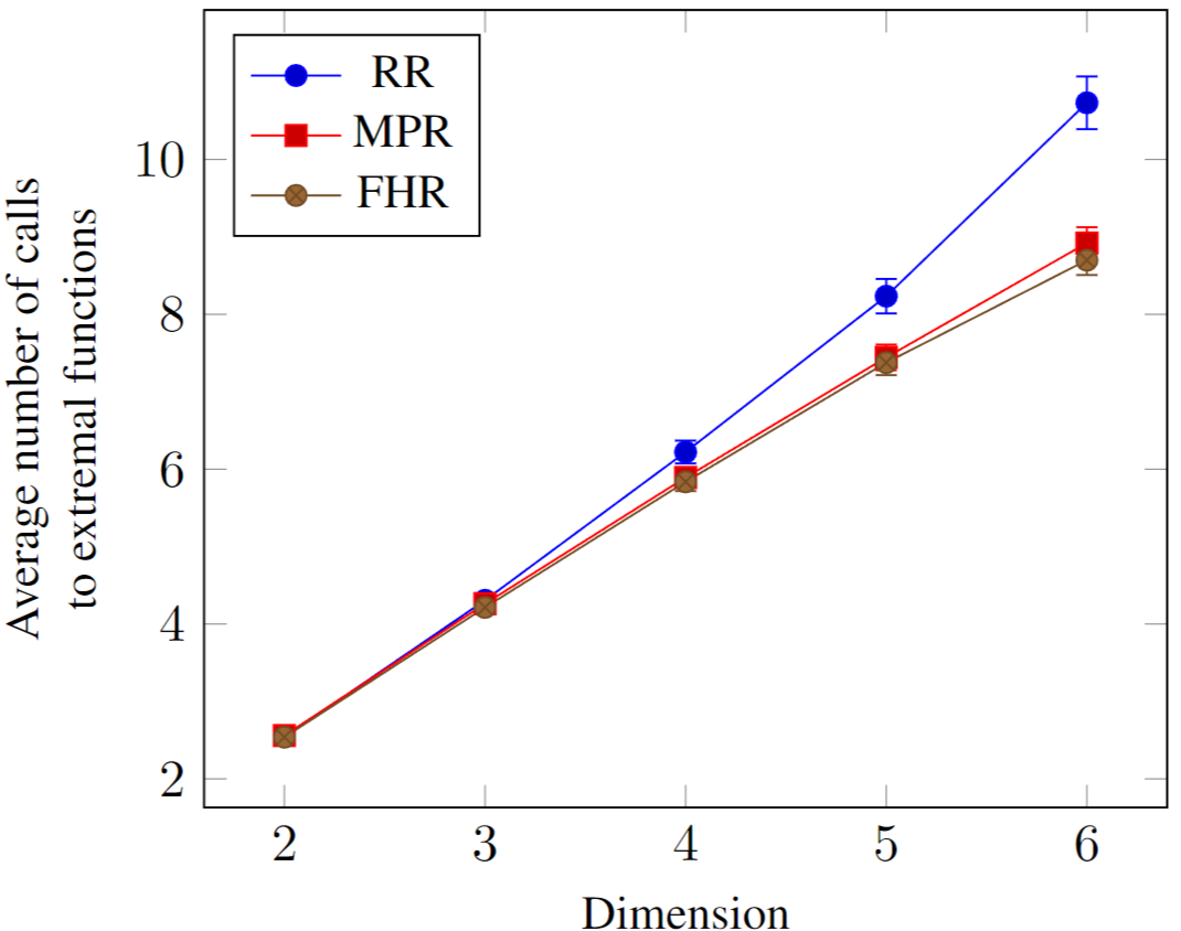
Figure 3. Performance of the three pivot rules. The error bars represent 95% confidence interval.

To see how much FHR outperformed compared with MPR, the following table shows the percentage of tests where FHR performed better, as good, and worse than MPR in terms of number of calls to extremal functions. We can see that FHR often outperformed MPR, but with not significant percentage of the time. Moreover, the gain when FHR performs better is smaller than the loss when it does worse. Therefore, it is inconclusive which method is better. Nonetheless, we chose FHR for simplicity and not in looking for a better method. This result is promising and deserves closer studies in the future.

$d$	2	3	4	5	6
Better	16.9%	18.6%	20.8%	21.65%	23.56%
As good	67.2%	64.4%	59.65%	57.55%	56.85%
Worse	15.9%	17.0%	19.55%	20.9%	19.5%
$\Delta\_{\text{better}}$	1.66	2.01	2.43	3.06	3.60
$\Delta\_{\text{worse}}$	1.68	2.09	2.56	3.28	3.90

Table 1. Comparison of performance for FHR and MPR. $\Delta\_{\text{better}}$ and $\Delta\_{\text{worse}}$ denote the gain and loss in number of extremal function calls when FHR performs better and worse, respectively.

5. Complexity assuming termination

From the mathematical description, it is clear that for $\sigma_P$ always returning a vertex of $P$ for any query, e.g. as an optimization oracle in linear programming problem, then suppose the algorithm terminates, the number of iterations is linear with respect to the number of vertices. Or in other words, if the algorithm terminates, one has that the complexity to be $O(\|\vertex{P}\|)$.

In this section, we will show that this bound is tight, and moreover, independent of the dimension. We shall assume the real computation model, i.e. numbers are represented with infinite precision, and for the sake of brevity, we shall outline only the key ideas of the construction.

The first key observation is how to construct such a polygon in 2-dimensional space. In this part, we shall use capital letters to denote points, and assume a plane without any coordinate systems.

Let $d$ be a line on which we choose an arbitrary point $A_0$. We take another point $A_1 \not\in d$, and draw the line $d_1$ passing through $A_1$ and perpendicular to $d$. Let $B_1$ be the intersection between $d$ and $d_1$. Then, on the halfplane defined by $d_1$ and containing $A_0$, we take another point $A_2$ such that the line segment $A_1 A_2$ intersects $A_0 B_1$. The triangle $A_0 A_1 A_2$ now gives our initial 2-simplex.

Then, let $d_2$ be the line parallel to $A_0 A_1$ and passing through $A_2$, and let $B_2$ be the intersection between $d_1$ and $d_2$. Since the line $d$ passes through the line segment $A_1 A_2$, it divides the triangle $\triangle A_1 A_2 B_2$ into two halves. We choose a point $A_3$ strictly in the interior of the half containing $A_1$.

And the process continues indefinitely. To be more precise, let $i \geq 2$, we draw the line $d_i$ passing through $A_i$ and parallel to $A_{i-2} A_{i-1}$, and let $B_i$ be the intersection between $d_{i-1}$ and $d_i$. Since the line $d$ passes through the line segment $A_{i-1} A_i$, it divides the triangle $\triangle A_{i-1} A_i B_i$ into two halves. We choose a point $A_{i+1}$ strictly in the interior of the half containing $A_{i-1}$.

Now let $n \geq 3$, we claim that

The points $A_0, A_1, ..., A_{n+1}$ are vertices of $P = \conv{\{A_0, A_1, ..., A_{n+1}\}}$. Indeed, for each $i > 0$, one has the line $d_i$ separates the plane into two halves, one of which contains $P$, and since $A_i \in d_i$, $A_i$ is a vertex of $P$. As for $A_0$, one can see that the line $d_0$ passing through $A_0$ and parallel to $A_1 A_2$ serves the same purpose.
The line $d$ intersects all triangle $A_i A_{i+1} A_{i+2}$ for all $i \geq 0$, since it intersects $A_i A_{i+1}$ for all $i > 0$.
Let $X$ be a point inside the triangle $\triangle A_{n-1} A_n A_{n+1}$ and lying on $d$, then the algorithm would take $n$ iterations even if we incorporate the information of $x$ in Phase 1, and regardless of the pivot rule. The conclusion follows.

What needs to be done is to generalise this construction to higher dimensions. One of the simple ways to do so in $\mathbb{R}^{d+1}$ is to take an arbitrary 2-dimensional subspace $H$ in which we carry out the above construction, and $d-1$ points $C_0, C_1, ..., C_{d-1}$ such that, for instance, the vectors $\overrightarrow{A_0 C_i}$ for $0 \leq i \leq d-1$ forms a basis of the complementary subspace $H^\perp$. Then, one has $P = \conv{\{A_0, A_1, ..., A_{n+1}, C_0, C_1, ..., C_{d-1}\}}$ is a non-degenerate polytope, and the analysis above holds, with the number of iterations remains $n$. An intuitive reason is because if we suppose a line $\ell \subseteq H$ separates two points $A, B \in H$ in $H$, then the affine hyperplane containing $\ell$ and $C_0, C_1, ..., C_{d-1}$ also separates two points $A$ and $B$ in $\mathbb{R}^{d+1}$.

Figure 4a. Construction in 2D...

Figure 4b. ...which is then lifted to 3D.

6. Conclusion

I present a mathematical description of a family of methods for the relative position problem, which involves initiating a simplex given by points on the boundary of the concerned polytope $P$ and gradually refining the simplex, until no such improvement can be done, at which point we can conclude about the relative position of $x$.

We also give definition of a pivot rule, and demonstrate the dependence of performance, and even of termination of the scheme on the choice of such a rule. Unfortunately the scope of the study does not allow further examination of the rules.

Finally, assuming the algorithm is executed in real computation model and terminates, we show that the complexity is linear in the number of vertices of $P$, and that this bound is tight, independent from the dimension. Note that in the context of RNA secondary structure, the polytope has potentially vertices exponentially many with respect to the number of features.

References

-- NGUYEN Doan-Dai , on September 11th, 2024